GPU Accelerated Offline Features

At Chalk, the federated query engine is one of our core products. It serves online features at low latency or runs large scale offline queries at high throughput to generate training datasets. We are approaching the limit of CPU performance for our offline queries after already having exploited vectorised instructions and multi-core parallelism. Given that we are always looking for the frontier of efficiency and performance, we started exploring how these workloads would run on a processor better built to handle parallelism.

In this post we dive into some of our insights from using GPUs to accelerate dataset generation with Velox’s cuDF implementation. This acceleration will enable researchers and data scientists to iterate faster when developing their ML models. We began by investigating where GPUs have the most impact with controlled experiments, and then applied these learnings to real production workloads that demonstrated significant performance gains.

How are queries run on a GPU?

Chalk’s Engine relies on a query planner to run queries. Our planner models customers’ feature definitions as a DAG (Directed Acyclic Graph) of relations. When a user submits a query, the planner constructs a logical plan to evaluate the desired output features from given inputs. The next layer of the plan takes this logical plan and lowers it into a physical Velox, an open source query execution engine, plan to define how a query runs on computers.

A query plan in Velox is defined as a tree of relational operators. Each operator represents a transformation on a row vector, such as an aggregation or a sort. Once Chalk has determined which fragments of our physical plan are GPU worthy, the Velox cuDF adapter replaces eligible operators with cuDF operators that perform their transformations on a GPU instead of CPU.

A Velox cuDF Operator follows the same interface as their CPU counterparts while differing in implementation:

• They apply transformations on device-native (that is, GPU native) cuDF Vectors.
• Each cuDF Vector also provides a CUDA stream.

A cuDF-backed operator translates its Velox operation into one or more cuDF calls—a filter for example. cuDF schedules the corresponding CUDA kernels on the vector’s stream and returns device-resident output buffers to be consumed by the next cuDF Operator.

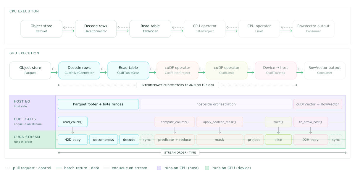
Figure 1: Velox query’s execution model on CPU vs GPU

As with most GPU programs, there is a tradeoff between fitting a dataset on device memory while giving hardware enough work to saturate compute. Next, we ran some experiments to see how this tradeoff mapped onto analytical query workloads. All experiments were performed on an NVIDIA RTX PRO 6000 Blackwell GPU.

When does GPU execution pay off?

We ran some TPC-H like queries through our execution engine to build an intuition for when GPU execution is worth its cost. TPC-H is a standardised set of queries often used to benchmark analytical database systems. These benchmarks allow us to make controlled variants in input size, data transformations, and result cardinality. We measured end-to-end execution times on these queries and collected traces using NVIDIA’s Nsight to answer:

• How to move and maintain data on a GPU during a query?
• What kind of operations is a GPU best suited for?
• What kind of operations are worse off on GPU than CPU?

Experiment 1: Moving data to the GPU

We receive input data in the form of Parquet files that need to be decoded before running a query. Velox gives us two options to do this:

• Host side scan: Decoding the parquet file in host memory and transferring the uncompressed bytes to device memory.
• Device side scan: Transferring the compressed Parquet file to device memory and performing the decode operation natively.

Intuitively, the device-side scan seems attractive because it will move fewer bytes while also leveraging GPU parallelism for repetitive decoding operations.

We ran a benchmark with 1.75 GiB of Parquet data on TPCH-Q07 comparing the two configurations and measured data transferred, host-to-device (H2D) transfer counts and payload sizes, and query time:

Unfortunately, reducing the number of bytes transferred alone did not offset the cost of these many H2D transfers. The cost of the overhead of the device-native decode operations outweighed the benefits of a smaller H2D transfer. While GPU-native scanning transferred less data, it issued more H2D transfers with smaller 49KB payloads, versus fewer H2D transfers averaging 720 KB for a CPU scan. Each payload warrants its own set of decompression and decode kernels, and the CUDA kernel launches needed to do that work are expensive.

The question then becomes, how can we reduce the number of transfers while maintaining the same number of bytes transferred? If we reorganize our input data into fewer but larger Parquet shards of the same dataset, we can have fewer decode kernels with each of them having more meaningful work.

We reran the same experiment but with a new layout for input data: 1.75 GiB split into 8 shards. We reduced end-to-end runtime from 9.73s to 6.66s—a 32% improvement. The following graph from Nsight traces validates our hypothesis:

The trace confirms that producing fewer but larger pieces of work results in meaningful performance gains. H2D and D2H movements reduced by 88%. The number of kernel launches also fell by 89% while SM util went up by 62%. Unlike a CPU, if we setup our input data into fewer but larger chunks, we get more efficient decode kernels and less runtime overhead.

Experiment 2: Finetuning parallelism

Now that we have our data loaded on device, we can start to reason about how operations on it should be executed.

In Velox, the number of drivers controls the number of concurrent batches that are processed. A Velox driver is a single thread that executes a pipeline of operators. Therefore, one way to control parallelism of query execution is through the number of drivers.

On GPU however, increasing driver count may not always improve throughput of a query. A single driver’s kernel launch could make use of all the streaming multiprocessors on the device! Conversely, additional drivers with multiple concurrent pipelines can lead to contention for device memory and other compute resources. Hence, one must find a balance between compute saturation and hardware resource contention when scheduling work on GPUs. Sweeping across driver counts TPCH-Q07 show us the following:

Moving from one to two drivers produced no material runtime improvement, while four drivers increased runtime nearly twofold and introduced substantial variability. The traces show that four drivers introduced significantly more memory operations.

Unified-memory host-to-device migrations increased from and device-to-host migrations rose more than thirteenfold. The runtime was spending more time maintaining data residency across concurrent producers, rather than executing the query.

This shows that the right driver count is dependent on the shape of the query and that we should strive towards finding the smallest value that hides scan and scheduling gaps while avoiding memory-residency contention.

Experiment 3: The cost of UVM

NVIDIA’s Unified Virtual Memory (UVM) model lets CPU and GPU programs refer to managed allocations through a single virtual address space. A buffer can remain addressable by both sides even when its pages reside only in host memory or only in device VRAM. When a GPU operator accesses a host-resident page, CUDA can migrate it to the device. This capability seemed promising for a hybrid engine like Chalk’s. CPU and GPU stages can pass logical buffers without requiring application code to manage explicit ownership handoff, and queries can address working sets larger than VRAM.

However, the driver-count experiments showed that extra concurrency can cause memory churn rather than throughput when using UVM. To understand why, we looked at how memory is managed across CPU and GPU execution with different allocation strategies. We started with queries whose working datasets fit on device memory. For TPCH-Q06, which has a smaller memory footprint than our TPCH-Q07 run in the previous sections since it does not include a hash join, we compared a device native allocation strategy (async) against using UVM apis for managing device memory (prefetched-managed):

Using the device native allocation strategy was 2.12x faster. Since neither configuration required oversubscription of device memory, there is likely significant overhead of maintaining migration-capable allocations. Traces for the same confirm our hypothesis:

While we can't directly compare these runtimes with those from Figure 6 due to the overhead from Nsight tracing, we can see that for the UVM based allocation configuration (prefetched managed), the GPU idles more compared to the device native allocation (async) config.

This cost compounds when a higher concurrency expands the active working set of a query beyond device memory. Re-visiting the TPCH-Q07 workload from the previous section, examining more memory traces justifies our reasoning:

UVM transfer volume increased more than tenfold along with the cumulative time spent in the `cudaMemPrefetchAsync` API time across all threads. This is the main tradeoff that shaped the rest of our tuning work: it is critical to maintain the active working set across all drivers in device memory to avoid expensive repeated page fault thrash.

Why joins make this harder

Joins keep their build-side hash table in GPU memory throughout the probe phase. Unlike scan buffers, which can be released after use, the hash table’s buckets, keys, payloads, and supporting buffers must remain available. Adding more drivers means more probe buffers and more hash-table pages accessed at the same time. When this combined memory footprint exceeds available VRAM, UVM must repeatedly move pages in and out of GPU memory. This creates more memory traffic without increasing useful throughput.

The practical implication is that join-heavy GPU queries need concurrency to be tuned against their resident hash-build footprint. They cannot use the same driver count as other operators simply because the GPU has available compute capacity.

Production Workloads

Our experiments established the operating conditions for effective GPU execution: feed the device sufficiently large units of work to offset runtime overhead and that we must tune concurrency to the query’s memory footprint. Let’s see if these learnings proved to be useful by testing on some real world use cases:

• A high cardinality aggregation representing behavior patterns for fraud detection.
• A compute intensive project and TopN reduction for search engine result ranking.

Ordered Aggregations for Fraud-Detection

This workload computes hourly behavioral features for fraud detection. For every user and hour, it distinguishes buyer vs. seller activity and calculates metrics like transaction counts, gross volume, type breakdowns, and activity timestamps. These feed fraud signals that track changes in user behavior and marketplace participation, making it a valuable dataset to train a model for fraud detection.

This workload groups user activity into millions of groups (one per user-hour pair) and tracks multiple aggregate states within each. High-cardinality grouping and complex state management are expensive on CPU but naturally parallelizable on GPU. The query executes as:

When we first ran this on the GPU, it did not scale as well as CPU execution with increasing row counts:

Profiling the 4B input run revealed a new bottleneck: the intermediate state from the partial aggregation was responsible for several D2D copies that accounted for a large portion of the GPU's runtime!

Partial aggregation is flushed frequently, producing wide intermediate rows that had to be materialized, repartitioned, and merged—an expensive operation for the GPU. We increased `max_partial_aggregation_memory` to retain more local state before flushing, reducing intermediate data volume at the cost of higher peak memory usage.

Increasing partial aggregation limit from 16 MiB to 6 GiB reduced our runtime from 290.1s to 53.2s. Profiling confirms our hypothesis: The partial aggregation step emits far fewer rows and we spend significantly less time making device-to-device copies.

Beyond 6 GiB, memory pressure outweighed savings (7 GiB) or caused OOM (8 GiB), establishing this as the operating point for another end-to-end measurement.

The new results validate our experiment, we see an almost 8x speedup and 500M inputs and 3.1x speedup for 4B inputs compared to 0.57x from earlier.

Projected Top-N for Search Engine Results Ranking

This workload ranks search candidates using relevance, personalization, conversion, and quality signals, producing a top-50 dataset that trains a downstream ranking model. The reranking projection performs roughly 390 scalar arithmetic operations per candidate to score them, before selecting the Top-50 listings, providing substantial independent computation across input rows that can benefit from GPU parallelism. The massive reduction to 50 output rows keeps memory usage and data movement minimal.

At 1B candidate listings (49.4 GiB of Parquet input), GPU execution completed in 6.96 seconds, an 11.2× speedup when compared with CPU execution!

Conclusion

GPUs can dramatically speed up queries, but it is not always a magic bullet. Compute-heavy workloads with large aggregations, projections, and TopN operations can run more than 10x faster. But inefficient data layouts or excessive data movement can erase those gains. We’re continuing to work on GPU-accelerated queries at Chalk. Stay tuned for more.